
Monte Carlo forecasting is the most common form of probabilistic forecasting that we see. It’s compelling because it can provide a highly accurate forecast of when work will be done, with relatively little effort.
For an overview of probabilistic forecasting as a whole, and why you might use it, see this article.
If you just want to use Monte Carlo to get a forecast, then you don’t need to know what I’m covering here. On the other hand, if you’re not sure if you can trust the forecast because you don’t understand how it works, this article is for you.
The problem
Let’s first consider what problem we’re trying to solve. Based on historical throughput data, we want to forecast how long it will take to complete a certain amount of new work.
For example, we have 11 weeks of weekly throughput data (how many items completed that week) as shown in this table. We have somewhere between 100 and 120 new items that need to be done.
| Week | 1 | 2 | 3 | 4 | 5 | 6 | 7 | 8 | 9 | 10 | 11 | 12 |
|---|---|---|---|---|---|---|---|---|---|---|---|---|
| Throughput | 1 | 3 | 5 | 3 | 7 | 8 | 0 | 5 | 3 | 1 | 8 | 2 |
The Monte Carlo simulation will give us an answer of the form “with 85% certainty, we’ll be done on or before October 1st”
One pass through
Monte Carlo is a simulation based approach, so we’re going to start with one simulation.
We know that we have between 100 and 120 items to do, so we’re going to roll the dice and pick a random number in that range. A random selection gives us 105.
Next we see that there are 12 weeks of throughput data, so we’ll randomly select a week and use the data for that week. Our random selection is week 8, and in that week we completed 5 items. We’ll subtract those 5 from our total of 105 work items, and now we have 100 work items remaining.
We randomly picked the week, and from that, determined the throughput. We did not randomly select a throughput value.
We then pick another random week (4) and see that we’d completed 3 items that week. So we subtract that 3 from our new remaining count. Now we have 97 work items left.
Do it again and again until there are no items remaining. The number of times we had to select a random throughput is the number of weeks that we expect it will take to complete all the work.
Let’s imagine that it had taken us 23 times through the loop to get the remaining count to zero. That means that this one run through the simulation predicted that it would take us 23 weeks to complete the work.
I expect at this point you’re already thinking that this is ridiculous, that we’re playing entirely with random numbers and that there can’t be any accuracy to this prediction at all.
If all we were doing was this one simulation run, then you’d be right.
Running multiple passes through the simulation
Now that we have the result from one simulation run, we start all over and do it again. Pick a random number of total items from the initial range of 100-120. Loop through randomly selected throughputs until we get a prediction of how many weeks it will take.
And then do it again. And again.
We’ll do this thousands of times, perhaps a million times. Once we have all of these samples together, we start looking at probabilities. If we graphed all of these thousands (or millions) of projections, we’d see a bell curve like the one below. The more samples we had, the smoother the curve of the bell would be.
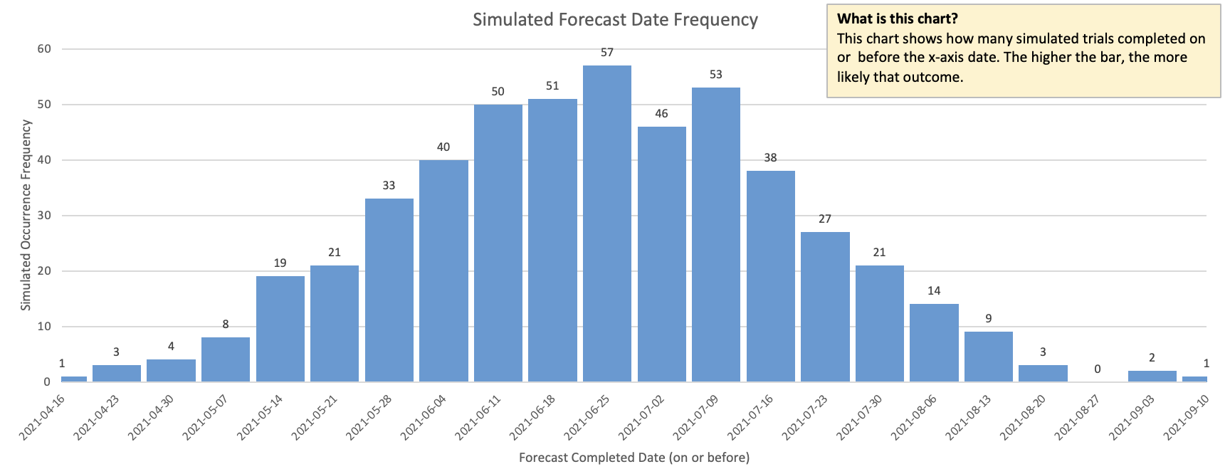
While each individual simulation run by itself was unpredictable, by looking at thousands of them together, we’re able to see clear patterns.
In this diagram, we can see that about half of them completed on or before June 25. Phrased as a forecast, we can say that with 50% probability, we’ll be done on or before June 25.
50% isn’t very accurate though. That’s a coin toss and it’s unlikely that your customers are willing to accept a forecast that’s only as accurate as a coin toss. At the same time, 100% certainty is impossible as there is always some uncertainty. The percentage that I tend to focus on is 85% as that tends to be the sweet spot of accurate enough. In practice, I find 85% to be extremely accurate.
In this case, 85% might be July 23.
So when we create a forecast with Monte Carlo, we’re saying that over the thousands of simulation runs that we did, 85% of them completed by this date, and assuming that future throughput is the same as past throughput, this forecast will be highly accurate.
Another variation
In the example above, we were specifically determining the date for a given amount of work. We can use exactly the same simulation approach if we wanted to determine how many items we could complete by a given date, and sometimes this is useful.
Example: We must deploy our mobile app by December 15 to ensure it’s in the app store by Christmas. How much work can we complete before that date?
Data quality
A similar approach is often used for weather prediction, and can be drawn in a Spaghetti Plot as shown in this picture from Weather.com.
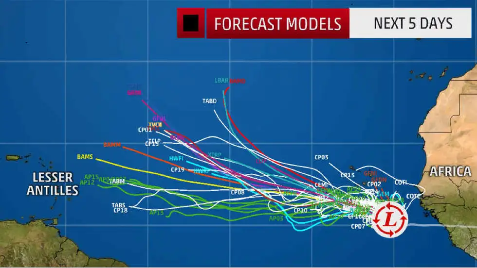
The danger with this forecast, is that we have to have historical data that is fundamentally predictable. Imagine that our weather spaghetti diagram looked like the one below. That data is fundamentally unreliable and any forecast we make off it will also be unreliable.
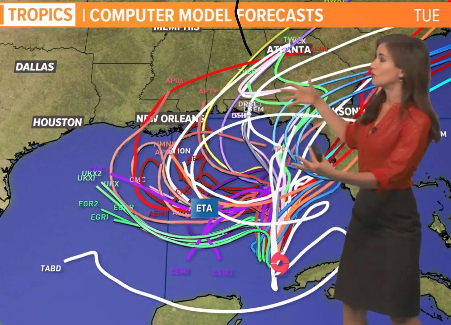
I’ve talked about making your data more reliable before and won’t get into that again. It’s critical to have good input data however.
Conclusion
If you do have good data, then a Monte Carlo forecast is a very low-effort way to get a highly accurate forecast. “Low effort” does imply that you’re using a tool to do this; you would never calculate this by hand.
The two Monte Carlo tools I use most often are the Throughput Forecaster from FocusedObjective.com (look under free tools) and Actionable Agile from 55 Degrees. You can’t go wrong with either one of these.